An Unbiased View of Vlookup Not Working
Use VLOOKUP when you need to discover things in a table or an array by row. For instance, search for a cost of a vehicle component by the part number, or find a worker name based upon their worker ID. In its simplest type, the VLOOKUP function states: =VLOOKUP(What you intend to search for, where you desire to seek it, the column number in the array consisting of the worth to return, return an Approximate or Exact suit-- suggested as 1/TRUE, or 0/FALSE).
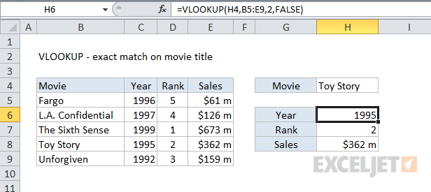
Use the VLOOKUP feature to look up a value in a table. Phrase structure VLOOKUP (lookup_value, table_array, col_index_num, [range_lookup] For instance: =VLOOKUP(A 2, A 10: C 20,2, REAL) =VLOOKUP("Fontana", B 2: E 7,2, FALSE) =VLOOKUP(A 2,'Client Information'! A: F,3, FALSE) Argument name Description lookup_value (called for) The value you intend to look up. The value you intend to look up have to be in the first column of the range of cells you define in the table_array debate.
Lookup_value can be a value or a referral to a cell. table_array (called for) The variety of cells in which the VLOOKUP will look for the lookup_value and the return value. You can make use of a called range or a table, as well as you can utilize names in the disagreement instead of cell recommendations.
The cell variety likewise requires to consist of the return worth you want to discover. Discover how to pick ranges in a worksheet. col_index_num (required) The column number (starting with 1 for the left-most column of table_array) which contains the return worth. range_lookup (optional) A sensible value that defines whether you desire VLOOKUP to locate an approximate or a precise suit: Approximate match - 1/TRUE thinks the initial column in the table is sorted either numerically or alphabetically, and will certainly after that look for the closest worth.
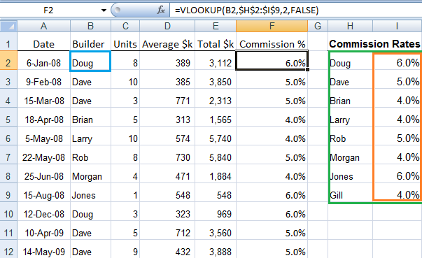
For example, =VLOOKUP(90, A 1: B 100,2, REAL). Precise suit - 0/FALSE searches for the specific worth in the very first column. For instance, =VLOOKUP("Smith", A 1: B 100,2, FALSE). There are 4 items of details that you will certainly need in order to build the VLOOKUP syntax: The value you want to look up, also called the lookup value.
Not known Facts About How To Vlookup
Remember that the lookup worth need to always be in the initial column in the array for VLOOKUP to function properly. For instance, if your lookup worth remains in cell C 2 then your variety ought to begin with C. The column number in the variety that includes the return worth. For instance, if you define B 2:D 11 as the array, you should count B as the first column, C as the 2nd, and more.
If you don't define anything, the default value will certainly always be TRUE or approximate suit. Now place all of the above together as complies with: =VLOOKUP(lookup worth, range including the lookup worth, the column number in the array having the return worth, Approximate match (TRUE) or Precise match (FALSE)). Below are a few examples of VLOOKUP: Issue What went incorrect Wrong value returned If range_lookup holds true or left out, the initial column requires to be arranged alphabetically or numerically.
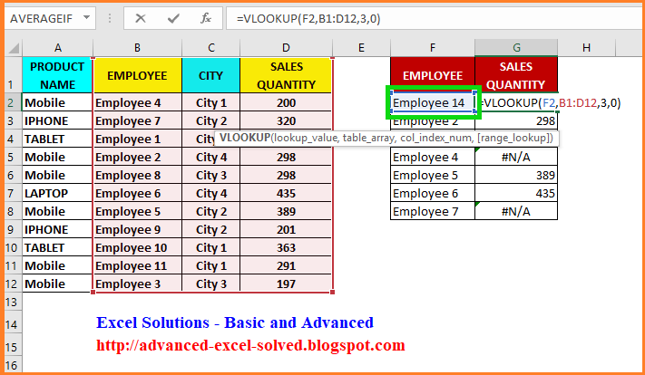
Either sort the first column, or utilize FALSE for a specific match. #N/ A in cell If range_lookup holds true, after that if the worth in the lookup_value is smaller than the smallest value in the very first column of the table_array, you'll get the #N/ An error value. If range_lookup is FALSE, the #N/ A mistake worth shows that the exact number isn't located.
#REF! in cell If col_index_num is more than the number of columns in table-array, you'll get the #REF! error value. To learn more on solving #REF! errors in VLOOKUP, see How to fix a #REF! error. #VALUE! in cell If the table_array is much less than 1, you'll get the #VALUE! mistake value.
#NAME? in cell The #NAME? error worth usually implies that the formula is missing quotes. To seek out a person's name, make certain you use quotes around the name in the formula. For instance, enter the name as "Fontana" in =VLOOKUP("Fontana", B 2: E 7,2, FALSE). For even more info, see How to fix a #NAME! mistake.
The Definitive Guide to How To Vlookup
Learn how to use outright cell recommendations. Don't store number or day worths as text. When looking number or date worths, make sure the information in the initial column of table_array isn't stored as message worths. Or else, VLOOKUP may return an inaccurate or unanticipated worth. Arrange the very first column Type the initial column of the table_array before using VLOOKUP when range_lookup is TRUE.


An inquiry mark matches any solitary personality. An asterisk matches any type of sequence of personalities. If you wish to locate an actual enigma or asterisk, type a tilde (~) before the personality. For instance, =VLOOKUP("Fontan?", B 2: E 7,2, FALSE) will browse for all instances of Fontana with a last letter that can vary.
When searching text worths in the first column, see to it the data in the first column doesn't have leading rooms, routing areas, irregular use of straight (' or") as well as curly (' or ") quote marks, or nonprinting characters. In these cases, VLOOKUP may return an unexpected value.
You can constantly ask a specialist in the Excel User Voice. Quick Recommendation Card: VLOOKUP refresher course Quick Referral Card: VLOOKUP repairing tips You Tube: VLOOKUP videos from Excel community specialists Every little thing you need to understand about VLOOKUP Exactly how to correct a #VALUE! error in the VLOOKUP feature Just how to remedy a #N/ An error in the VLOOKUP function Summary of formulas in Excel Exactly how to stay clear of broken formulas Identify errors in formulas Excel features (indexed) Excel features (by category) VLOOKUP (complimentary sneak peek).
To determine shipping price based on weight, you can utilize the VLOOKUP feature. In the instance revealed, the formula in F 8 is: =VLOOKUP(F 7, B 6: C 10,2,1)* F 7 This formula utilizes the weight to find the appropriate "price per kg" after that ... To bypass result from VLOOKUP, you can nest VLOOKUP in the IF feature.
excel vlookup not found excel vlookup in russian vlookup in excel from another tab